ETL with AWS Glue
Transforming the data with Glue
The dataset that we ingested using Lake Formation had a schema design that had been optimized for a traditional relational database. For example, there is a customer table and a separate customer_address table, and these are linked using a foreign key. Similarily there is a web_sales table and a separate items table, where each web_sale links via a foreign key to an item in the items table.
For the ETL job in this lab we are optimizing our customer data for use by our marketing department who want to analyze the dataset for different marketing campaigns at the state level. They have indicated that some of their campaigns will also be targeting different sets of customers based on whether they live in a single family house, an apartment, or a condo.
Our ETL job will:
- Denormalize our customer data by joining the customer and customer_address tables
- Drop a number of columns that our marketing department does not need
- Rename columns to remove the naming references to the original table
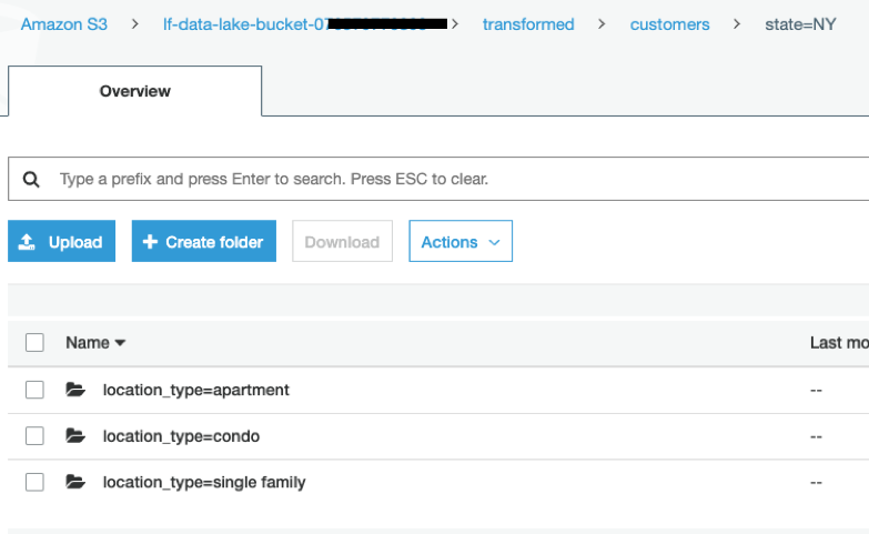
- Write out the new customers table to a new transformed location in S3, with the data partitioned by State and Location Type (Single Family, Apartment, Condo).
Open the notebook and review the ETL code
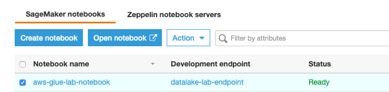
On the left-hand side of the Glue console, click on Notebooks (under Dev endpoints) and confirm that the notebook you created has a status of Ready.
Click the selector box next to the newly created notebook (such as aws-glue-lab-notebook) and then click the Open notebook button
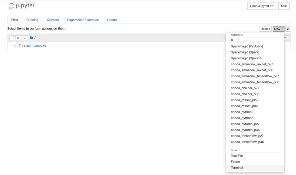
On the right-hand side of the Jupyter notebook screen, click on the New dropdown and then click Terminal
Copy and paste the following commands into the terminal window. This will download the Jupyter notebook (.ipynb extension) that contains the code for this lab.
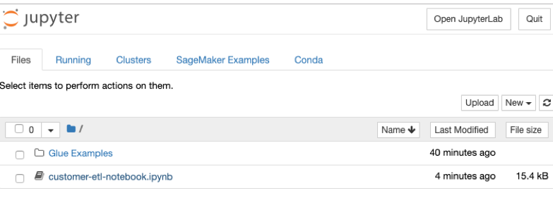
cd SageMaker

wget lakeformation-lab.s3-website-us-east-1.amazonaws.com/customer-etl-notebook.ipynb
Close the browser tab with the terminal, and go back to the tab containing the Jupyter notebook. You should now see the customer-etl-notebook.ipynb file. Click on this file to open it.
In Jupyter notebooks, you are able to have separate blocks of code and run one block at a time, with the server response / output displayed directly below the box. In this notebook, the first block of code imports various Glue libraries and initializes a Spark session.
Click in the first block, and then click the Run button inside the top toolbar.
Notice how to the left of the block, the In [ ] changes to In [*] while the code is running, and then finally to In [1] once the code completes. The number indicates the order that you have run the code blocks in. Output that the code generates is listed below the code block, and the focus is automatically moved to the next block
Now run the second block of code, again by clicking on the Run button in the toolbar.
Continue running the subsequent blocks of code, except for the last block, one at a time (wait until the code has finished executing before running the next block).
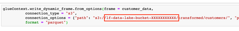
The last block of code will write out the transformed data to our data lake, partitioned by state and location_type, under the prefix transformed. Before running this, you need to edit the code to specify the name of your bucket (which you can get from the CloudFormation output from the first lab, or by going to the S3 console and looking for the bucket name that begins with lf-data-lake-bucket-…..
Replace the path in the marked area below with the name of your bucket, and then run this block of code.
Once this code block completes, open up the S3 service in the AWS management console, and browse to the transformed location and view the partitions and files.